Markovian Ducks Riddler
Two Friday’s ago, the FiveThirtyEight Riddler problem asked us to consider some ducks stochastically swimming between rocks in a pond. We are told that initially the ducks are sitting together on a rock in the middle of the pond, and each minute all of the ducks will independently randomly swim to one of their neighboring rocks with equal probability. We are told to assume that the rocks are laid out in a square grid, and that the ducks only swim horizontally and vertically. Assuming \(2\) ducks on a \(3 \times 3\) grid, the prompt asks us: how long on average will it take for all of the ducks to land together on the same rock?
As usual, the bonus question is to generalize the problem. In particular, we’ll consider \(k \geq 2\) ducks on an \(m \times m\) grid (for \(m\) odd).
In this post I’ll walk through my thought process for solving this problem and provide some solutions for small numbers of ducks and rocks. I wrote some code to both solve this problem numerically and to estimate the result by simulating the random process. This code can be found here.
Process Illustration
Before solving the problem I thought it would be fun to visualize things. The following animation illustrates the process for \(k\) ducks (depicted by yellow circles) on an \(m \times m\) grid of rocks. When the ducks arrive on the same rock, they’ll briefly turn green before the process restarts in the middle.
Solving for Average Duck Meeting Times
Because the only information that the ducks use to select their next rock is which rocks are adjacent to their current rock, and since the ducks each swim independently of one another, we can initially consider each ducks’ behavior independently as a discrete Markov process on a graph with \(m \times m\) vertices. The next step will be to modify the process so that the joint process is absorbing when the ducks are in the same state, and finally to solve a certain linear system to obtain the average time for the ducks to meet.
Single Duck Transitions
We start by considering a single duck on a \(m \times m\) grid. Let’s index the rocks (since we’ll implement this numerically in the end) and let \(i\) denote the index of the rock that the duck is currently standing on. Letting \(X_n\) denote the single duck’s random walk, and \(N(i)\) denote the set of neighboring cells, the single duck transition matrix has the following form:
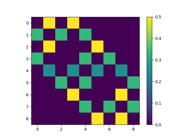
\[P^{(1)}_{ij} = P(X_{n+1} = j | X_n = i) = \left\{\begin{array}{lr} \frac{1}{|N(i)|} & \text{if $j \in N(i)$} \\ 0 & \text{else} \end{array}\right.\]For ducks on a \(3 \times 3\) grid, if we index the rocks from left to right and top to bottom as in the following table.
| 6 | 7 | 8 |
| 3 | 4 | 5 |
| 0 | 1 | 2 |
The resulting single-duck transition matrix has the following appearance.
Multiple Duck Transitions
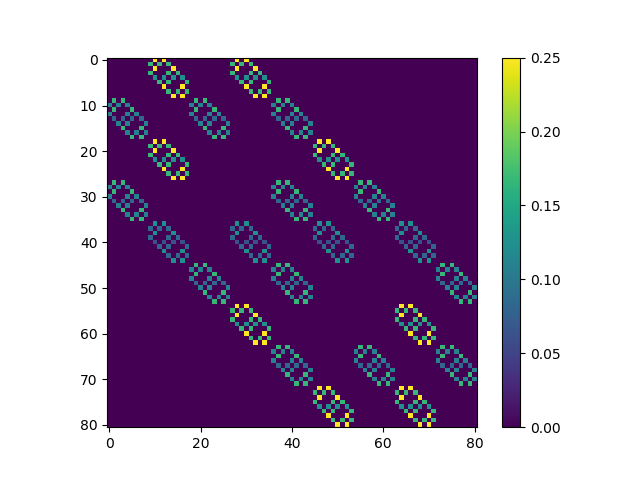
Since each duck transitions independently according to the same Markov process, the \(k\)-duck transition matrix is simply the tensor product of the \(k\) single-duck transition matrices. That is,
\[\begin{eqnarray} P^{(k)}_{(i_1,\ldots,i_k), (j_1,\ldots,j_k)} &=& P(X^{(1)}_{n+1} = j_1, \ldots, X^{(k)}_{n+1} = j_k | X^{(1)}_n = i_1, \ldots, X^{(k)}_{n+1} = i_k) \\ &=& P^{(1)}_{i_1 j_1} \cdots P^{(1)}_{i_k j_k} \end{eqnarray}\]If we flatten the \(k\) indices as follows \((i_1,\ldots,i_k) \mapsto \sum_{j=1}^{k} (m^2)^{k-1} \cdot i_k\) then the \(2\)-duck transition matrix for a \(3 \times 3\) grid has the following appearance:
Absorbing States
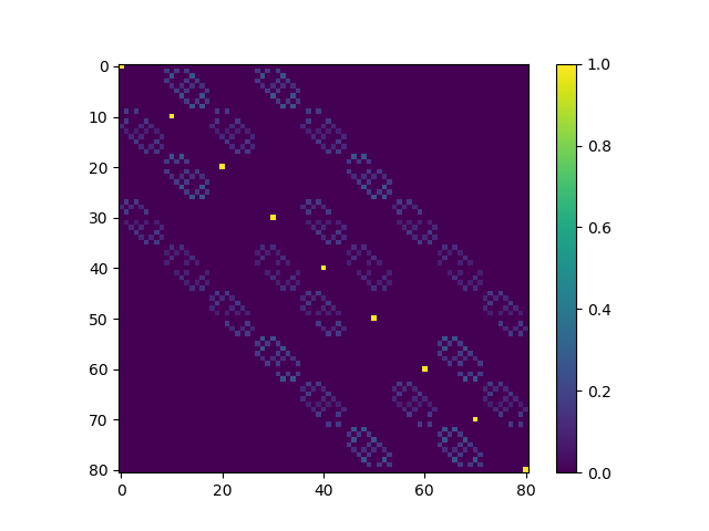
Next, we will modify the \(k\)-duck Markov process so that the states where the ducks come together are absorbing. To do this, we just set
\[Q^{(k)}_{(i_1,\ldots,i_k),(j_1,\ldots,j_k)} = P^{(k)}_{(i_1,\ldots,i_k),(j_1,\ldots,j_k)}\]if the \(i_l\) are not all equal, otherwise
\[Q^{(k)}_{(i,\ldots,i), (j_1,\ldots,j_k)} = \left\{ \begin{array}{lr} 1 & \text{if $j_1 =\ldots=j_k$} \\ 0 & \text{else} \end{array}\right.\]Put differently, to form \(Q^{(k)}\) we take the \(k\)-duck transition matrix \(P^{(k)}\), and then we zero-out the rows where \(i_1 =\ldots = i_k\) while setting the on-diagonal entry in those rows to be \(1\).
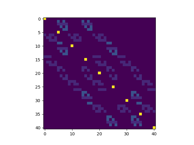
For \(2\) ducks on a \(3 \times 3\) grid, this results in the following modified transition matrix.
Inaccessible States
Before proceeding to compute the mean absorption time, we will want to make one additional simplification to the transition matrix \(Q^{(k)}\). Recall that our Markov process starts with all ducks sitting on the same middle rock. The ducks then swim to a neighboring rock according to \(P^{(k)}\) and the process proceeds from there according to \(Q^{(k)}\). Because all of the ducks are together at time \(n=0\), and only move horizontally or vertically by one cell, it is easy to see that the difference between the sum of each pair of ducks’ \(x\) and \(y\) coordinates is divisible by \(2\). This will remain true after every step in the Markov process. As a consequence, some states of the transition matrix \(Q^{(k)}\) are not reachable from our process.
The following image shows shows the graph described by the transition matrix for \(2\) ducks on a \(3 \times 3\) grid. In particular, we see that index \(0\) and \(1\) belong to disjoint components of the graph, so \(0\) is not reachable from \(1\) and vice-versa. Here \(0\) corresponds to one of the absorbing states, and it can be shown that all of the absorbing states are reachable from the initial position.
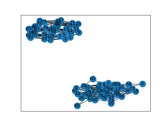
We do not need to worry about unreachable states, so they should be removed from the matrix \(Q^{(k)}\). In fact, for computational efficiency we shouldn’t even bother to compute the entries of the matrix \(Q^{(k)}\) for those states! Due to laziness, my implementation currently does not use this simplification and instead proceeds to compute \(Q^{(k)}\) and to use the graph described above to select the reachable states.
A reduced transition matrix \(\widetilde{Q}^{(k)}\) for transitions to the accessible states can obtained by excluding the inaccessible states and re-indexing the matrix. For \(2\) ducks on a \(3 \times 3\) grid, the resulting reduced matrix looks as follows.
Notice that there are half as many rows in this matrix. For \(k \geq 2\) ducks the reduction is in even greater (so I’m performing a lot of wasted effort by not removing these states)!
Mean Time to Absorption
Let \(T_A\) denote the time at which the process described by \(\widetilde{Q}^{(k)}\) is absorbed, and let \(\mu^{(k)}\) be the column vector of expected absorption times from transient states, i.e. \(\mu^{(k)}_i = E[T_A | X_1 = i]\), where \(i\) is a transient state. A standard result from the theory of discrete-time Markov processes is that if all states are either absorbing or transient (which is the case for \(\widetilde{Q}^{(k)}\)), then \(\mu^{(k)}\) can be computed by solving a certain linear system.
To define the linear system, let \(R^{(k)}\) to be the submatrix of \(\widetilde{Q}^{(k)}\) formed by including only the rows and columns corresponding to transient states. Then \(\mu^{(k)}\) can be computed by solving
\[(I - R^{(k)}) \mu^{(k)} = \mathbf{1}\]where \(\mathbf{1}\) is a column vector consisting entirely of ones.
The final step is to compute the expected absorption time \(E[T_A]\) from the initial state at time \(t = 1\) and to add one to the result to get the total expected steps. See that
\[E[T_A] = \sum_i E[T_A | X_1 = i] \cdot P^{(k)}(X_1 = i) = \sum_i \mu_i \cdot P_{ii_0}\]where \(i_0\) is the state where all the ducks are in the middle square. The final results is then
\[1 + \sum_i \mu^{(k)}_i \cdot P^{(k)}_{ii_0}.\]Results
The following table shows the result of solving the above linear system and simulating the Markov process for \(k = 2, \ldots, 5\) ducks for grids with \(m = 3,5,\ldots,9\) rocks per row. Results are only shown when the matrix \(Q^{(k)}\) had fewer than \(60,000\) rows (since my current implementation could only handle problems of that size). The simulated mean was computed by averaging the stopping time from \(10,000\) simulated \(k\)-duck Markov processes.
| Rocks Per Row | Number of Ducks | Simulated Mean | Solved Mean |
|---|---|---|---|
| 3 | 2 | 4.858 | 4.9054 |
| 3 | 3 | 18.208 | 18.4360 |
| 3 | 4 | 66.8171 | 66.7420 |
| 3 | 5 | 236.6482 | 237.3955 |
| 5 | 2 | 14.4637 | 14.6696 |
| 5 | 3 | 146.7471 | 149.7365 |
| 7 | 2 | 29.7964 | 29.7727 |
| 9 | 2 | 51.0354 | 50.0824 |