Inefficient Cranberry Sauce Passing Riddler
In this post, I’ll walk through my solution to last week’s cranberry sauce passing problem from FiveThirtyEight’s “The Riddler.” In this problem, we’re asked to consider 20 guests sitting around a circular Thanksgiving table, who all want to receive a serving of cranberry sauce. These guests are somewhat lazy/careless, and whenever a guest receives the sauce, they will randomly pass the sauce to their left or right with equal probability. The guests continue in this fashion until everyone has been served. Under these conditions, we are asked:
- Assuming that the sauce begins in front of a pre-specified guest, which of the remaining guests has the greatest chance of receiving the sauce last?
The answer to this problem is different from what you might expect (I definitely did not anticipate it), however, the distribution doesn’t make a very interesting plot. Since I’m mostly interested in making pretty graphs, I decided to consider the following related problems:
- How long should we expect the process to take, and how much more inefficient is this process than direct passing?
- How much longer should we expect the process to take if a given guest is the last person to receive the sauce?
To solve these problems, I considered cranberry sauce passing as a pair of discrete Markov processes. One process, the primary chain, was used to track the guests who had already been served, while the other process, the auxiliary chain, was used to model how the sauce is passed before reaching the next unserved guest. In solving these problems, I also chose to consider an arbitrary number of guests, since it didn’t require much extra work.
Jupyter notebooks for my solutions can be found in this github
repository. In
one notebook
(compute_analytical_solution.ipynb),
I provide solutions for Problems 1-3 using some standard (and one less
standard) theoretical results about Markov chains with absorbing
states. A second notebook
(run_simulation.ipynb)
is provided, in which I run a straightforward simulation of the process
to serve as a cross-check of my analytical solution. The simulation
results are designed to run in parallel in a fully reproducible fashion –
which is something I hadnt’t accomplished in the past. So, if you
happen to have a computer with at least 16 cores, you should be able to
reproduce my results verbatim 🙂
Cranberry Passing Markov Process
In order to determine who is last to be served, we only really need to track the order in which guests are served. We can ignore the intermediate left/right passes which occur amongst guests who have already been served. With this in mind, we can model cranberry sauce passing as a discrete Markov process whose states reflect which guest has been served most recently, and which guests have already been served. For a table with 6 guests, the states can be depicted as follows:
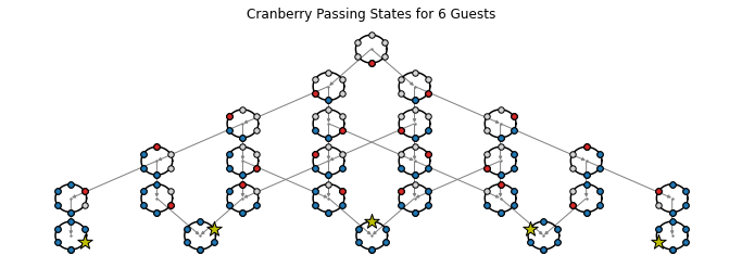
In this image, white dots reflect guests who have not been served yet, and blue dots are used to denote guests who have already been served. Red dots are used to denote the most recently served guest whenever unserved guests remain, while gold stars are used to indicate a guest who is served last. Small arrows have been drawn between states to indicate the possible transitions.
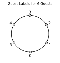
Before labeling the states of the Markov process, we first index the guests who are seated around the table. Let \(0\) denote the guest who will begin the process. Note that guest \(0\) can never be served last, unless they are the only guest. The remaining guests are enumerated counter-clockwise from guest \(0\), so that guest \(1\) sits to the right of guest \(0\), guest \(2\) sits to the right of guest \(1\) and so on. Letting \(n_{guests}\) denote the number of guests, it follows that guest \(n_{guests} - 1\) will be sitting to the left of guest \(0\). As an example, here’s what the labeling scheme looks like for a table with \(6\) guests:
To label the states of the cranberry passing Markov chain, we will use
the following notation. For non-terminal states (which are states for
which there are still unserved guests), we will use labels of the form
(last_served, served_interval, n_served). Here last_served denotes
the guest who was served most recently, served_interval is a
two-tuple whose entries are the two previously guests who are
respectively seated furthest to the left and right of guest \(0\).
The third state component, n_served is provided for convenience in
my computational implementation (it isn’t really necessary) and
reflects the number of guests in served_interval. Finally, since
we’re not concerned with the direction from which the sauce arrives to
the last guest, we simply label terminal states (states where the
final guest is served) with the index for the guest who is served
last.
Using this notation, the states for a table with 6 guests can be depicted as follows:
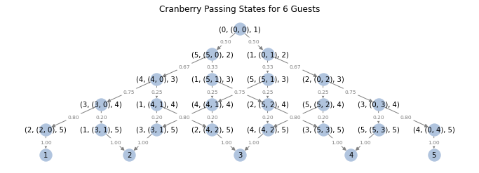
In the image above, I have indicated the probabilities for each transition, which will be discussed in the next section.
Transition Probabilities
To determine the transition probabilities, we now introduce an
auxiliary Markov chain, which tracks the left/right passes through the
interval of guests which have previously been served, up until the
time when the sauce escapes the interval from the left or from the
right. This kind of process is referred to colloquially as a
“Drunkard’s Walk” for a finite interval. In our case, the walker in
the process begins on one edge of the finite interval (with length
n_served) and takes steps to the left or right with equal
probability. Under these conditions, it can be shown (see e.g. this
discussion)
that the walk will eventually exit the interval, and that it will exit
through the edge nearest or furthest from the initial edge with
probabilities:
Thus for transitions to non-terminal states, the cranberry passing Markov chain transition probabilities are given by:
\[P(S_{t+1} = S_j | S_{t} = S_i) = \left\{ \begin{array}{cl} \frac{n_{\text{served}} - 1}{n_{\text{served}}} & S_j = S_{\text{near}, i} \\ \frac{1}{n_{\text{served}}} & S_j = S_{\text{far}, i} \\ 0 & \text{else} \end{array} \right.\]Where, if the walk begins on the left edge of served_interval, that
is, if \(S_i =
(\text{left},~(\text{left},~\text{right}),~n_\text{served})\) then
If the walk begins on the right edge, that is, if \(S_i = (\text{right},~(\text{left},~\text{right}),~n_\text{served})\), then the formulas for \(S_{i, \text{near}}\) and \(S_{i,\text{far}}\) are exchanged. Note that we are identifying \(-1\) with \(n_{\text{guests}} - 1\) here.
Finally, transitions from states with \(n_\text{served} = n_{\text{guests}} -1\) to the terminal state corresponding to the final remaining guest occur with probability 1, and the cranberry passing process remains in these terminal states with probability 1.
To get a feel for how all of this shakes out, you might want to refer to the graph above, and inspect the transition probabilities listed along the graph edges. I have intentionally suppressed self-loops for the terminal states, so you won’t see those probabilities highlighted there (i.e. states \(1,\ldots,5\) should have loops back to themselves with a labels of 1 along each loop). Alternatively, you can have a look at the following figure, which shows the cranberry passing transition matrix as a heat-map:
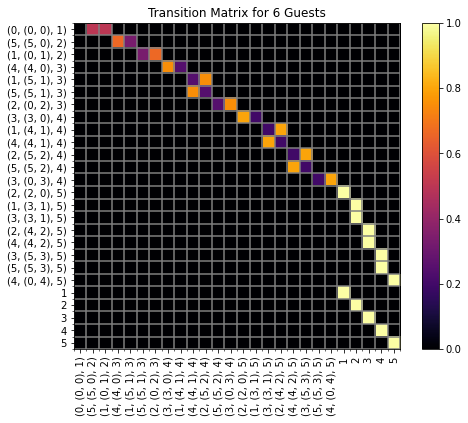
Although I like the aesthetic of the heat-map a bit better, I think it’s somewhat harder to parse than the other figure 🙂
As a final note, to build the transition matrix, we have to assign an indexing for the states. Since it simplifies things a bit to have the terminal states in the bottom right hand portion of the transition matrix, we employ the following iterative procedure to index the states. To begin the indexing, we first assign the starting state \((0,(0,0),1)\) with an index of 1. Then, for each \(n > 1\), we take the ordered list of states \(\Sigma_n\) having \(n_\text{served} = n - 1\) and form \(\Sigma_{n+1}\) by appending, for each \(S\in\Sigma_n\), the left and then right descendant states for \(S\) (here \(S'\) is the left descendant of \(S\) if \(S'\) is reached from \(S\) by passing to the left of the served interval, and is right descendant if it is reached by passing to the right). As a consequence of this construction, the terminal states (which correspond to \(n_\text{served} = n_\text{guests}\)) will end up on the lower-right most corner sub-matrix of \(P\). Essentially, we index the set of states by indexing each successive row left-to-right from top-to-bottom in the graph depicted above.
Solving Problem 1
As discussed in the preceding section, by construction, the transition matrix for the cranberry passing process has already been placed in canonical form (see e.g. Wikipedia). That is,
\[P = \left( \begin{array}{cc} Q & R\\ 0 & I_r \end{array} \right)\]Here \(r = n_\text{guests} - 1\) is the number of terminal states.
The probability that the Markov chain terminates in state \(j\) beginning from state \(i\) can be obtained from the \((i,j)\) entry of the matrix \(B\) where \(B\) solves:
\[(I - Q) B = R\]Since the cranberry sauce passing process begins from state \((0, (0,0), 1)\), we need only to consider the row associated with this state from the matrix \(B\), i.e. we need only consider the first row of \(B\).
Solving Problems 2 & 3
Solving Problem 3
We will solve Problem 2, to compute the unconditioned mean number of passes, by first solving Problem 3. That is, we begin by computing the mean number of passes conditioned on a specific guest being last.
To that end, let \(k \neq 0\) be one of the guests. We will compute the mean number of passes made, conditioned on \(k\) receiving the sauce last, by looking at all of the paths through the cranberry passing state-space which terminate with \(k\). For each such path, we can estimate the expected number of sauce passes by computing the expected number of passes associated with each transition in the path and summing the results together. Finally, we need only sum the path means together weighted by the conditional probability of each path given that \(k\) is served last.
To begin, let \(\Gamma_k\) denote the set of paths from \((0,(0,0),1)\) to \(k\), i.e.
\[\Gamma_k = \{S_1, \ldots, S_\text{n_guests} : S_1 = (0,(0,0), 1), S_{n_\text{guests}} = k, P_{S_{t+1}S_{t}} > 0~\text{for $t = 1,\ldots,n_{guests}-1$} \}\]We can compute:
\[E[N_\text{passes} | \text{$k$ is last}] = \sum_{\gamma \in \Gamma_k} E_\gamma[n_\text{passes}]\cdot P(\gamma | \text{$k$ is last})\]where \(E_{\gamma}[n_\text{passes}] = \sum_{i=1}^{n_\text{guests}} E[N_{\text{passes}, S_i, S_{i+1}}]\), and \(E[N_{\text{passes}, S_i,S_{i+1}}]\) is the expected number of passes when the sauce transitions from state \(S_i\) to state \(S_{i+1}\).
For the transitions to non-terminal states (i.e. \(i < n_\text{guests}-1\)), the last quantity, \(E[N_{\text{passes}, S_i,S_{i+1}}]\), is the expected number of steps until absorption in the Drunkard’s walk on an interval of length \(i\) described above, conditioned on this process starting on one edge and exiting from the near edge or far edge – depending on whether \(S_{i+1}\) is the near or far edge from \(S_i\). For the terminal transition (i.e. \(i = n_\text{guests}-1\)), we need the unconditioned mean number of steps until absorption when the Drunkard’s walk starts on one edge of a length \(n_\text{guests} - 1\) interval instead.
The unconditioned expectation is easy to compute and follows from standard results about absorbing Markov chains applied to the Drunkard’s walk on an interval of length \(n_\text{guests}-1\), see e.g. Wikipedia’s discussion on absorbing Markov Chains. The conditioned expectations for the non-terminal transitions are a bit trickier, but to compute the mean number of steps in the cases when the Drunkard’s walk terminates in either the near or far edge, one can apply Theorem 1 from this paper (which you can obtain here). In any event, to compute either the unconditioned or conditioned means, one needs only to solve a linear system associated with the transition matrix for the appropriate finite Drunkard’s walk.
The only remaining component is the probability \(P(\gamma |\text{$k$ is last})\). Let \(\gamma = (S_1,\ldots,S_{n_\text{guests}})\) be one of the paths in \(\Gamma_k\). The unconditioned probability of \(\gamma\) is simply \(P(\gamma) = \prod_{1}^{n_\text{guests} - 1} P_{S_iS_{i+1}}\), and since \(\Gamma_k\) contains all paths for which guest \(k\) is served last, the conditioned probability can be obtained by
\[P(\gamma | \text{$k$ is last}) = \frac{P(\gamma)}{\sum_{\alpha \in \Gamma_k} P(\alpha)}.\]With this, we have all the required ingredients to compute \(E[N_\text{passes} |\text{$k$ is last}]\).
Note: The method I have outlined here probably isn’t the simplest method possible… but it is the one I implemented. The set \(\Gamma_k\) can be very large, and likely has factorial growth in \(n_\text{guests}\) – so implementing the calculation as described above is fairly computationally intensive.
Solving Problem 2
The only remaining question to answer is how to compute the unconditioned mean number of passes. This can be done as follows:
\[E[N_\text{passes}] = \sum_{k=1}^{n_\text{guests} - 1} E[N_\text{passes} |\text{$k$ is last}] \cdot P(\text{$k$ is last})\]Essentially, to solve Problem 2, we just combine the solutions for Problems 1 & 3.
Solutions for \(n_\text{guests} = 20\)
Solution to Problem 1
The following figures shows the solutions to Problem 1 when \(n_\text{guests} = 20\).
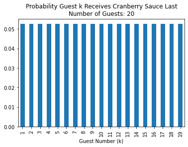
Note that the probability that guest \(k\) is last does not depend at all on where that guest is sitting! It really seems like guest 10, who is furthest away from where the sauce begins, should be more likely to be served last than guests 0 or 19, who are sitting right next to the guest who is served first. However this is not the case.
The solution for general \(n_\text{guests}\) appears to be the same. That is, the probability that guest \(k \neq 0\) is served last is uniform across \(k\). However, I only checked \(n_\text{guests} \leq 20\) and my solution requires solving a linear system to check the answer for a given \(n_\text{guests}\).
Solution to Problem 2
The average number of passes was found to be 190. In fact, it appears that for any \(n_{\text{guests}}\) the expected number of passes is \(\left(\begin{array}{c} n_\text{guests}\\ 2\end{array}\right) = \frac{n_\text{guests} \cdot (n_\text{guests} - 1)}{2}.\)
Since all \(n_\text{guests}\) could be served in as few as \(n_\text{guests} -1\) passes, we see that the cranberry passing process requires \(\frac{n_\text{guests} - 2}{2}\cdot 100\%\) more passes than necessary. For 20 guests, we can expect to observe 900% more passes than is necessary!
Solution to Problem 3
The following figures shows the solution to Problem 2 when \(n_\text{guests} = 20\).
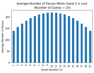
Note that, unlike the probability discussed in Problem 1, the conditioned average number of passes behaves like one would expect. That is, if the furthest guest from the starting point is served last (i.e. if guest 10 is served last), then we can expect the process to terminate in around 220 passes. This is substantially longer than when the last guest to be served is sitting next to the first served guest (e.g. when guest 1 is served last), when the process terminates in only 139 passes on average.
Average Number of Passes
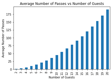
The following figures respectively show the average number of passes and the process inefficiency for \(n_\text{guests} = 2,\ldots,20\).
 |
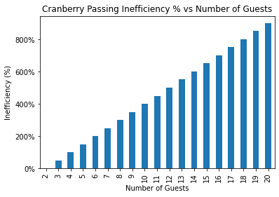 |
As mentioned above, it appears that that \(E[n_\text{passes}] = \frac{n_\text{guests} \cdot (n_\text{guests} - 1)}{2},\) and that inefficiency behaves like \(\text{Inefficiency}(n_\text{guests}) = \frac{n_\text{guests} - 2}{2}\cdot 100\%\).
Validating Analytical Results via Simulation
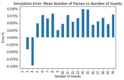
As mentioned in the introduction, I performed a simple stochastic simulation of cranberry passing to validate my theoretical calculations. For this simulation, I directly simulated cranberry sauce passes until every guest had been served. Simulations were conducted for \(n_\text{guests}=2,\ldots,20\), and for each \(n_\text{guests}\) the process was simulated \(10^6\) times.
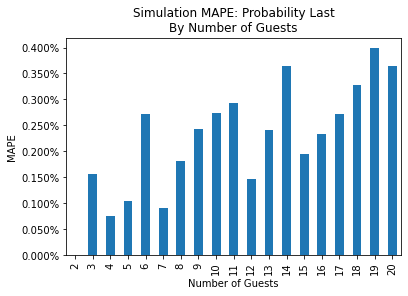
Since there was a high degree of accuracy for the simulated metrics of interest, I have only included aggregated error comparisons. The following figures compare the mean absolute percent error (MAPE) between the theoretical and simulation results for the probabilities (on the left) and for the simulated conditional means by number of guests (on the right).
 |
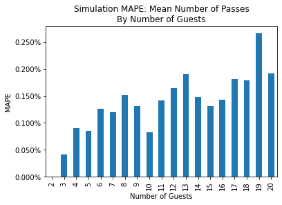 |
The following figure compares the mean percent error between the simulated and theoretical mean number of passes.