Groundhog Day T-Testing
While looking for some details on t-tests, I ran across this post from The Minitab Blog, which investigated Punxsutawney Phil’s powers of prognostication. The authors of that post tested whether there was a statistically significant difference in the average monthly temperature in the months immediately following Phil’s predictions when he saw his shadow vs when he didn’t. Detecting an increase in mean temperature when Phil saw doesn’t see his shadow would support Phil’s prognostication claims.
The original blog post used average temperature data for Pennsylvania over a 30 year period, but they were a bit opaque about the source of their data and didn’t have year labels on their data. As such, I thought I’d perform a similar analysis with a slightly clearer data lineage and longer history. Since I don’t use Minitab, I performed my analysis in Python.
For this analysis, I obtained monthly average temperature data from NOAA’s Global Summary of the Month for Jefferson County PA, which is where the borough of Punxsutawney is located. Phil’s predictions were sourced from the Wikipedia entry for Punxsutawney Phil, however the data provided there were originally sourced from Stormfax.com. The temperature data and Wikipedia page, both sourced in Apr-2020, can be found in this repository.
Here, we set up some package imports that we will use throughout.
import sys, os, re, requests, urllib3, pathlib
from bs4 import BeautifulSoup
import numpy as np
import pandas as pd
import seaborn as sns
import matplotlib.pyplot as plt
from scipy.stats import ttest_ind
from IPython.core.display import display, HTML
data_path = "./data/"
temperature_data_path = data_path + "/TempJeffersonCountyPA"
Punxsutawney Phil Data
Because I didn’t feel like copying down the data about Phil’s predictions by hand, we will use Beautiful Soup to extract the data from the Wikipedia summary. To begin, we will need to download the Wikipedia entry if we don’t already have it. The entry, downloaded on 04/17/2020, is included in the repository. (The page may have changed after that date, so it is included for reproducibility).
ghog_pred_html = data_path + "/wiki_phil.html"

if not os.path.exists(ghog_pred_html):
    url = "https://en.wikipedia.org/wiki/Punxsutawney_Phil"
    req = requests.get(url)
    req_text = req.text

    with open(ghog_pred_html, 'w') as f:
        f.write(req_text)

else:
    with open(ghog_pred_html, 'r') as f:
        req_text = "".join(list(f))
Next we parse the Wikipedia entry. Here, we build the soup and find the table containing Phil’s predictions.
# build the soup
soup = BeautifulSoup(req_text, 'html.parser')

# find the only wikitable, which has the prognostications
table = soup.find('table', {'class' : 'wikitable'})
table_rows = table.find_all('tbody')

# We can throw away the table caption, since it links to
# the original page
table.find("caption").decompose()
Next we’ll render the table that we extracted. The table doesn’t come with its legend, so we’ll also render it. Some minor modifications of the original HTML were necessary in order to make this look nice in my notebook.
# find the legend
legend = soup.find('div', attrs={'style' : 'float: left;'})
legend = legend.find("tbody")

# the legend was aligning right, so force it to align left
for div in legend.findAll("div", attrs={'class' : 'legend'}):
    div['style'] = 'text-align:left;'

# Render the html
display(HTML(table.prettify()))
display(HTML(legend.prettify()))
| 1887 | 1888 | 1889 | |||||||
| 1890 | 1891 | 1892 | 1893 | 1894 | 1895 | 1896 | 1897 | 1898 | 1899 |
| 1900 | 1901 | 1902 | 1903 | 1904 | 1905 | 1906 | 1907 | 1908 | 1909 |
| 1910 | 1911 | 1912 | 1913 | 1914 | 1915 | 1916 | 1917 | 1918 | 1919 |
| 1920 | 1921 | 1922 | 1923 | 1924 | 1925 | 1926 | 1927 | 1928 | 1929 |
| 1930 | 1931 | 1932 | 1933 | 1934 | 1935 | 1936 | 1937 | 1938 | 1939 |
| 1940 | 1941 | 1942 | 1943 | 1944 | 1945 | 1946 | 1947 | 1948 | 1949 |
| 1950 | 1951 | 1952 | 1953 | 1954 | 1955 | 1956 | 1957 | 1958 | 1959 |
| 1960 | 1961 | 1962 | 1963 | 1964 | 1965 | 1966 | 1967 | 1968 | 1969 |
| 1970 | 1971 | 1972 | 1973 | 1974 | 1975 | 1976 | 1977 | 1978 | 1979 |
| 1980 | 1981 | 1982 | 1983 | 1984 | 1985 | 1986 | 1987 | 1988 | 1989 |
| 1990 | 1991 | 1992 | 1993 | 1994 | 1995 | 1996 | 1997 | 1998 | 1999 |
| 2000 | 2001 | 2002 | 2003 | 2004 | 2005 | 2006 | 2007 | 2008 | 2009 |
| 2010 | 2011 | 2012 | 2013 | 2014 | 2015 | 2016 | 2017 | 2018 | 2019 |
| 2020 | |||||||||
Next we parse the table and use the table’s cell styles to determine whether Phil saw his shadow or not in each year. We will only retain the “Long Winter” (shadow) and “Early Spring” (no shadow) records, and will set all other records as missing.
# get all of the entries in the table, cell contents are years
# and style denotes if a shadow was seen or not
tds = table.find_all('td', style=True)
years  = [int(td.text) for td in tds]
styles = [td['style'] for td in tds]

# use the color coding to identify if a s
shadow = []
for s in styles:
    if "azure" in s:
        shadow.append(True)   # azure = SHADOW
    elif "gold" in s:
        shadow.append(False)  # gold = NO SHADOW
    else:
        shadow.append(np.nan) # sometimes no records, once war clouds

# Create a dataframe of the records
df_phil = pd.DataFrame({"year" : years, "shadow" : shadow})
df_phil = df_phil[~df_phil["shadow"].isnull()]
df_phil.head()
| year | shadow | |
|---|---|---|
| 0 | 1887 | True |
| 1 | 1888 | True |
| 3 | 1890 | False |
| 11 | 1898 | True |
| 13 | 1900 | True |
Temperature Data
NOAA’s site only allows you to export a certain number of records at a time, so I had to split my export into two separate requests. Weather data is (partially) available for Jefferson County from 1892 onward, so I requested all records from June-1892 through March-2020. The dataset I received contained monthly temperature records from multiple stations in Jefferson County. For this analysis we will primarily be interested in the average temperature “TAVG.” We’ll drop the other columns and rename those columns that we do keep.
temperature_data_files = os.listdir(temperature_data_path)
temperature_data_file_paths = [temperature_data_path + "/" + f for f in temperature_data_files]
df_temperature = pd.concat((pd.read_csv(f) for f in temperature_data_file_paths))

print("Data file names")
print("---------------")
for f in temperature_data_files:
    print(f)

# Build the data frame. Only retain average
df_temperature.columns = [c.lower() for c in df_temperature.columns]
df_temperature['date'] = pd.to_datetime(df_temperature['date'])
df_temperature = df_temperature[['station', 'date', 'tavg']]
df_temperature = df_temperature.rename(columns = {'tavg' : 't_avg'})
df_temperature = df_temperature.dropna()
df_temperature.head()
Data file names
---------------
jefferson_county_pa_temp_189206_195005.csv
jefferson_county_pa_temp_195006_202003.csv
| station | date | t_avg | |
|---|---|---|---|
| 0 | USW00014741 | 1926-01-01 | 22.0 |
| 1 | USW00014741 | 1926-02-01 | 23.6 |
| 2 | USW00014741 | 1926-03-01 | 28.3 |
| 3 | USW00014741 | 1926-04-01 | 40.0 |
| 4 | USW00014741 | 1926-05-01 | 53.9 |
Since we’re not especially interested in the individual stations’ average monthly temperature, we’ll average across stations to get a representative value for Jefferson County. Some additional columns are added for convenience later on.
df_montly_temperature = df_temperature.groupby('date').mean().reset_index()
df_montly_temperature['month'] = pd.DatetimeIndex(df_montly_temperature['date']).month
df_montly_temperature['year']  = pd.DatetimeIndex(df_montly_temperature['date']).year
df_montly_temperature = df_montly_temperature[['date', 'year', 'month', 't_avg']]
df_montly_temperature.head()
| date | year | month | t_avg | |
|---|---|---|---|---|
| 0 | 1896-09-01 | 1896 | 9 | 70.3 |
| 1 | 1896-10-01 | 1896 | 10 | 52.1 |
| 2 | 1896-11-01 | 1896 | 11 | 47.1 |
| 3 | 1897-01-01 | 1897 | 1 | 32.8 |
| 4 | 1897-02-01 | 1897 | 2 | 43.6 |
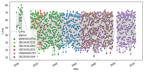
Here we provide a scatter-plot of the average temperature for each station and compare to the mean across stations, which is plotted as a solid line.
fig, ax = plt.subplots(figsize = (10,5))
df_montly_temperature.plot(x = 'date', y = 't_avg', ax = ax, c='k', alpha=0.25)
sns.scatterplot(x='date', y='t_avg', hue='station', data=df_temperature, ax=ax)
plt.show()
Next we create a dataframe of the average temperature for February and March of each year. Some years were missing records for either February or March, so we’ll exclude those years from our analysis. The mean for the two months is then computed as the simple average of each month’s mean. In doing this, we are ignoring the fact that February has fewer days than March. A more careful analysis would not neglect this fact, but this should be good enough for our purposes. 🙂
df_feb_mar_avg = (df_montly_temperature[(df_montly_temperature['month'] == 2) | (df_montly_temperature['month'] == 3)]
               .groupby('year')[['t_avg']]
               .agg(['count', 'mean']))
df_feb_mar_avg.columns = ['_'.join(col).strip() for col in df_feb_mar_avg.columns.values]
df_feb_mar_avg = df_feb_mar_avg.reset_index()
df_feb_mar_avg = df_feb_mar_avg[df_feb_mar_avg['t_avg_count'] == 2]
df_feb_mar_avg = df_feb_mar_avg[['year', 't_avg_mean']]
df_feb_mar_avg = df_feb_mar_avg.rename(columns = {'t_avg_mean' : 't_avg'})
df_feb_mar_avg.head()
| year | t_avg | |
|---|---|---|
| 0 | 1897 | 47.05 |
| 3 | 1900 | 29.10 |
| 4 | 1901 | 24.45 |
| 6 | 1911 | 32.95 |
| 7 | 1912 | 24.45 |
2-Sample Mean t-test
Finally we’ve got all of the data that we will need for the t-test. Let’s merge the two dataframes together and throw away any years in which we are missing either a temperature measurement or a prediction from Phil.
df_combined = pd.merge(df_phil, df_feb_mar_avg, left_on = "year", right_on = "year", how = "outer")
df_combined = df_combined.dropna()
df_combined.head()
| year | shadow | t_avg | |
|---|---|---|---|
| 4 | 1900 | True | 29.10 |
| 5 | 1901 | True | 24.45 |
| 15 | 1911 | True | 32.95 |
| 16 | 1912 | True | 24.45 |
| 17 | 1913 | True | 33.85 |
Let’s take a quick look at the mean temperature for Feb-March in years when Phil saw his shadow, as compared to the mean in years when he didn’t see his shadow.
df_combined.groupby('shadow').agg({'t_avg' : ['count', 'mean']})
| t_avg | ||
|---|---|---|
| count | mean | |
| shadow | ||
| False | 16 | 30.596875 |
| True | 89 | 30.176966 |
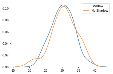
The means are pretty similar, so I wouldn’t expect our t-test to report a significant difference. Next we’ll convert the temperature to vectors for the t-tests, plot the distribution of the means in each prediction class, and then we’ll run the t-test. In the t-test, we’ll assume the samples have the same variance, although Scipy can run a test that allows for different variance between the different populations.
avg_temp_shadow    = df_combined[df_combined['shadow'] == True ]['t_avg'].to_numpy().flatten()
avg_temp_no_shadow = df_combined[df_combined['shadow'] == False]['t_avg'].to_numpy().flatten()
sns.distplot(avg_temp_shadow,    hist=False, label="Shadow")
sns.distplot(avg_temp_no_shadow, hist=False, label="No Shadow")
plt.show()
ttest_rslt = ttest_ind(avg_temp_shadow, avg_temp_no_shadow,
                       equal_var=False)

print("T-Test Result")
print("-------------")
print("t-value: {}".format(ttest_rslt.statistic))
print("p-value: {}".format(ttest_rslt.pvalue))
T-Test Result
-------------
t-value: -0.4104841358882534
p-value: 0.6859415624804476
The test shows that we failed to reject the null hypothesis that the two means were equal. As such, we cannot conclude that the means are different, but we also cannot conclude that the means are equal. That being said, it seems fairly likely that the means are the same, which reduces my confidence in Phil’s prognostications a little bit. 🙂