Poisson Spam Riddler
In this post, I’ll walk through a solution to FiveThirtyEight’s Riddler Classic problem from last week. In this problem, we are asked to consider a spam comment generation process. In this process, spam replies will respond to an initial post and to each subsequently generated spam reply. Spam will accumulate on each post/reply according to identical independent Poisson processes with a common rate of one comment per day (refer to the original prompt for a more clear explanation). We are asked: how many spam posts can we expect to have after three days?
My solution will consist of two parts. First, I’ll give an exact solution (although some details will be left “to the reader”), and then I’ll simulate the result to validate my exact solution. Finally, a comparison of the results will be provided at the end.
For reference, I have copied the verbatim below:
Last week’s Riddler column garnered six comments on Facebook. However, every single one of those comments was spam. Sometimes, spammers even reply to other spammers’ comments with yet more spam. This got me thinking.
Over the course of three days, suppose the probability of any spammer making a new comment on this week’s Riddler column over a very short time interval is proportional to the length of that time interval. (For those in the know, I’m saying that spammers follow a Poisson process.) On average, the column gets one brand-new comment of spam per day that is not a reply to any previous comments. Each spam comment or reply also gets its own spam reply at an average rate of one per day.
For example, after three days, I might have four comments that were not replies to any previous comments, and each of them might have a few replies (and their replies might have replies, which might have further replies, etc.).
After the three days are up, how many total spam posts (comments plus replies) can I expect to have?
Exact Solution
Throughout this discussion, we will let \(X_n\) denote the random interrarival time between the \((n-1)^{th}\) and \(n^{th}\) spam comments (for notational convenience, we let \(X_0 = 0\) denote the start of the process). We will let \(S_n\) denote the time of the \(n^{th}\) arrival, which is just the sum of the inter-arrival times, \(S_n = \sum_{k=1}^n X_k\). To keep things a bit more general than in the original prompt, we’ll let \(\lambda\) denote the per-comment spam arrival rate, and let \(T\) denote the time window during which we observe spam arrivals. We will let \(N(T)\) denote the number of spam comments that we observe by time \(T\). To be pedantic, we also point out that \(N(T)\) is a random variable that takes on non-zero integral values (it represents a count after all 🙂). With this notation in mind, the problem statement can be rephrased as: compute \(E[N(T)]\).
To compute \(E[N(T)]\), we will proceed as follows:
- Specify the distribution of the interarrival times \(X_n\) for \(n \geq 1\). [See here]
- Directly compute \(P(N(T) = n)\). [See here]
- Directly compute \(E[N(T)]\), by \(E[N(T)] := \sum_{n=0}^{\infty} n \cdot P(N(T) = n)\). [See here]
I haven’t considered whether there is a simpler approach to computing the expectation - there probably is, but I couldn’t think of a more clever solution!
Density of \(X_n\)
Once there are \(n-1\) comments/replies, the \(n^{th}\) spam post will either be a response to either the initial post or one of the \(n-1\) comments/replies. Since responses to each post/comment/reply arrive according to indepedent identical Poisson processes, each with rate \(\lambda\), we see that \(X_{n}\) will be the minimum of \(n\) i.i.d. \(\text{Exp}(\lambda)\) random variables. Thus, by a standard fact about the minimum of i.i.d. exponential R.V.’s, we have:
\[X_{n} \sim \text{Exp}(n\lambda) \text{ for $n \geq 1$}.\]Letting \(f_n\) denote the p.d.f. for \(X_n\), and \(F_n(t)\) its c.d.f., then for \(t \geq 0\) we have:
\[f_n(t) = (\lambda n) e^{-\lambda n t}\]and
\[F_n(t) = 1 - e^{-\lambda t}\]Computing \(P(N(T) = n)\)
Computing \(P(N(T) = n)\) is tedious but tractable in general. I will “leave it to the reader” to fill out the general case, but will compute the exact value for \(n=0,1,2\) (basically, I couldn’t think of a clever trick to quickly obtain the general case).
Case \(n = 0\)
Note that \(N(T) = 0\) just in case \(S_1 = X_1 > T\). Thus \(P(N(T) = 0) = P(X_1 > T) = 1 - (1 - e^{-\lambda T})\) so,
\[P(N(T) = 0) = \boxed{e^{-\lambda T}}\]Case \(n = 1\)
Note that \(N(T) = 1\) just in case \(S_1 = X_1 \leq T\) and \(S_2 = X_2 + X_1 > T\). So:
\[\begin{array}{rl} P(N(T) = 1) &= P\left(X_1 \leq T\text{ and }X_1 + X_2 > T \right)\\ &=\int_0^T f_1(t)\cdot P(t + X_2 > T)\,dt\\ &=\int_0^T f_1(t)\cdot P(X_2 > T - t)\,dt\\ &=\int_0^T f_1(t)\cdot (1 - F_2(T - t))\,dt\\ &=\int_0^T \lambda e^{-\lambda t}e^{-2\lambda(T - t)}\,dt\\ &=e^{-2\lambda T}\int_0^T \lambda e^{\lambda T}\,dt \\ &=\boxed{e^{-\lambda T}\cdot (1 - e^{-\lambda T})} \end{array}\]Case \(n = 2\)
Note that \(N(T) = 2\) just in case \(S_2 = X_1 + X_2 \leq T\) and \(S_3 = X_1 + X_2 + X_3 > T\). So:
\[\begin{array}{rl} P(N(T) = 2) &= P\left(X_1 + X_2 \leq T\text{ and }X_1 + X_2 + X_3 > T \right)\\ &=\int_0^{T} \int_0^{T - t_1} f_1(t_1)\cdot f_2(t_2)\cdot P(t_1 + t_2 + X_3 > T)\,dt_2\,dt_1\\ &=\int_0^{T} \int_0^{T - t_1} f_1(t_1)\cdot f_2(t_2)\cdot (1 - F_3(T - t_1 - t_2))\,dt_2\,dt_1\\ &=\int_0^{T} \int_0^{T - t_1} \lambda e^{-\lambda t_1} \cdot 2\lambda e^{-2\lambda t_2}\cdot e^{-3 \lambda (T - t_1 - t_2)}\,dt_2\,dt_1\\ &=e^{-3 \lambda T}\int_0^T \int_0^{T - t_1} \lambda e^{2\lambda t_1} \cdot 2\lambda e^{\lambda t_2} \,dt_2\,dt_1\\ &=e^{-3 \lambda T}\int_0^T 2\lambda e^{2\lambda t_1} \int_0^{T - t_1} \lambda e^{\lambda t_2} \,dt_2\,dt_1\\ &=e^{-3 \lambda T}\int_0^T 2\lambda e^{2\lambda t_1} (e^{\lambda(T-t_1)} - 1) \,dt_1\\ &=2 e^{-2 \lambda T} \int_0^T \lambda e^{\lambda t_1} \,dt_1 - e^{-3 \lambda T}\int_0^T 2\lambda e^{2\lambda t_1} \,dt_1\\ &=2 e^{-2 \lambda T} (e^{\lambda T} - 1) - e^{-3 \lambda T} (e^{2\lambda T} - 1)\\ &= e^{-\lambda T} - 2e^{-2 \lambda T} + e^{-3 \lambda T}\\ &=\boxed{e^{-\lambda T}\cdot (1 - e^{-\lambda T})^2} \end{array}\]General \(n\) (by hand-waving)
The pattern above allows us to conjecture that, in general:
\[\boxed{P(T(N) = n) = e^{-\lambda T} \cdot (1 - e^{-\lambda T})^n}\]This should be possible to verify pretty easily, but I didn’t bother to do it. We will, however, proceed as if I had verified it 🙂.
Computing \(E[N(T)]\)
The hand-waving above gave us that \(P(N(T) = n) = e^{-\lambda T} \cdot (1 - e^{-\lambda T})^n\). So we see,
\[\begin{array}{cl} E[N(T)] &= \sum_{n=0}^\infty n \cdot P(N(T) = n)\\ &= e^{-\lambda T} \cdot \sum_{n=1}^\infty n (1 - e^{-\lambda T})^n \\ &= e^{-\lambda T} \cdot \frac{(1 - e^{-\lambda T})}{(1 - (1 - e^{-\lambda T}))^2} \\ &= \frac{(1 - e^{-\lambda T})}{e^{-\lambda T}} \\ &= e^{\lambda T} - 1 \end{array}\]Here, we have computed the sum using the relationship between \(\sum_{n=1}^\infty nr^n\) and the derivative of a geometric series.
We have shown that the average number of spam comments by time \(T\) for a spam process of mean \(\lambda\) is:
\[E[N(T)] = e^{\lambda T} - 1\]For the case considered in the prompt, we have \(\lambda = 1\), and \(T = 3\), so the solution to the prompt is:
\[\boxed{E[N(T_{prompt})] = e^3 - 1 \approx 19.0855}\]Simulation Solution
In this section, we will simulate the spam process. Because I worked on this section before I reasoned through the exact approach, the approach we will consider here is a bit different from above. In particular, instead of utilizing the observation that the \(n^{th}\) inter-arrival time is an \(\text{Exp}(n\lambda)\) r.v. (which could have been used to generate more efficient simulations), I used the fact that responses to each comment/reply follow a Poisson process with rate \(\lambda\). This perspective can be accomodated by arranging responses according to the spam reply tree structure, that is, by organizing each spam reply according to which comment or post to which it is a reply.
To perform the simulation, we first simulate the number / time of each direct response that each post/comment/reply receives prior to time \(T\). This process is iterated for each child comment/reply and all of its descendant responses until we run out of descendant responses that arrive prior to time \(T\).
To simulate the number / time of direct responses that each post/comment/reply will receive, we use the standard approach described here. That is, we use the fact that the number of direct responses, \(N_c\), that a comment/reply/post created at time \(t\) will have in the window \([t,T]\) is a Poisson r.v., and that \(N_{c} \sim \text{Poisson}(\lambda \cdot (T - t))\). The arrival times for its children can then be simulated by generating \(N_c\) uniform R.V.’s on the interval \([t, T]\).
To simulate the total number of comments, direct responses are generated for each descendant response until we reach the point that a response has no descendants prior to time \(T\). The total number of comments is then found by counting all of the responses that were generated, which we compute recursively using the tree structure.
import numpy as np
from scipy.stats import poisson, uniform, linregress
import matplotlib.pyplot as plt
import seaborn as sns
import secrets
import networkx as nx
from networkx.drawing.nx_agraph import graphviz_layout
import pathos.multiprocessing as mp
import pandas as pd
Here we give a class to represent the spam comment trees. The spam tree itself is represented by a root node which has no parent.
class ResponseNode:
    def __init__(self, time=None, parent_id = None):
        self.parent_id = parent_id
        self.id = secrets.token_hex(nbytes=4)
        if time is None:
            time = 0
        self.time = time
        self.children = []

    def __str__(self):
        rslt = 'id: {} parent_id: {} time: {:0.05f}\tn_direct_children: {}\n'.format(
            self.id, self.parent_id, self.time, len(self.children))
        for c in self.children:
            rslt = rslt + c.__str__()
        return rslt

    def countChildren(self):
        if self.children:
            return len(self.children) + sum([c.countChildren() for c in self.children])
        else:
            return 0

    def addChildByTime(self, tc):
        childNode = ResponseNode(time = tc, parent_id = self.id)
        self.children.append(childNode)

        return childNode
The following function simulates the tree of spam comments for a single initial post.
def simulate_responses(Tf, respNode = None, mu=1):
    if respNode is None:
        respNode = ResponseNode()

    T0 = respNode.time
    responses = []
    n_comments = poisson.rvs(mu * (Tf-T0), size=1)
    t_comments = uniform.rvs(loc=T0, scale = (Tf-T0), size=n_comments)

    for t in t_comments:
        childNode = respNode.addChildByTime(t)
        simulate_responses(Tf, childNode, mu)

    return respNode.countChildren()
Tree example
Before proceeding, we give a simple visual example of the spam reply tree structure. To that end, the following function is used to graph a single spam tree. Note that this function is provided for visualization and does not impact the final simulation.
def graph_from_tree(node, G = None):
    if G == None:
        G = nx.Graph()

    #node_label = (node.id, '{0:0.4f}'.format(node.time))
    node_label = '{0:0.3f}'.format(node.time)

    if not G.has_node(node_label):
        G.add_node(node_label)

    for c in node.children:
        #child_label = (c.id, '{0:0.4f}'.format(c.time))
        child_label = '{0:0.3f}'.format(c.time)

        G.add_node(child_label)
        G.add_edge(node_label, child_label)

        graph_from_tree(c, G)

    return G
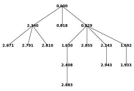
Here we provide a graph of a single spam tree on the window \([0,3]\). The numbers on the nodes represent the time that each comment/reply was created. The root node corresponds to the seed post, which is posted at the start time \(t = 0\).
# Generate a process
np.random.seed(1234)
rootNode = ResponseNode()
simulate_responses(Tf = 3, respNode = rootNode);

# Plot the process
G = graph_from_tree(rootNode)
pos = graphviz_layout(G, prog='dot')
nx.draw(G, pos, node_size=0, font_weight='bold', with_labels=True, arrows=False)

# How many children?
print("There were a total of {} spam replies in this simulation.".format(rootNode.countChildren()))
There were a total of 14 spam replies in this simulation.
Simulation
Now, we simulate the process for \(T = 1,\ldots,6\), with rate \(\lambda = 1 \text{ post / day}\). Due to inefficiency of the simulation and the exponential trend in the number of comments as \(T\) grows, we limit the number of simulations to \(50,000\) runs per final time \(T\).
n_simulations = 5e4
T_max = 6
%%time
sim_rslts = dict()
sim_means = dict()

for Tf in range(1, T_max + 1):
    with mp.Pool(12) as p:
        sim_rslts[Tf] = p.map(lambda x: simulate_responses(Tf = Tf),
                              np.arange(n_simulations))
        sim_means[Tf] = np.mean(sim_rslts[Tf])
CPU times: user 6 s, sys: 184 ms, total: 6.19 s
Wall time: 3min 45s
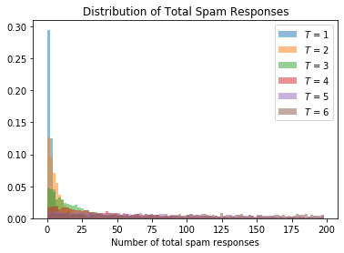
Just because we can, here’s a plot of the distribution of total spam responses for each \(T\) considered above. This plot shows that, for each \(T\), the probability that we observe \(n\) spam responses drops of exponentially in \(n\).
fig, ax = plt.subplots()

for Tf in range(1, T_max+1):
    ax.hist(sim_rslts[Tf], bins=np.arange(0,200,2), density=True, alpha=0.5, label="$T$ = {}".format(Tf))
ax.legend()
ax.set_title("Distribution of Total Spam Responses")
ax.set_xlabel("Number of total spam responses")
plt.show()
Results Validation
The following table compares the exact and simulated mean number of spam messages observed for each final time \(T = 1,\ldots,6\) with response rates \(\lambda = 1 \text{ comment/day}\). We see that the exact results are likely correct 🙂.
df_rslts = pd.DataFrame({'T' : list(sim_means.keys()), 'simulated_mean_spam_cnt' : list(sim_means.values())})
df_rslts['exact_mean_spam_cnt'] = np.exp(df_rslts['T']) - 1
df_rslts.style.hide_index()
| T | simulated_mean_spam_cnt | exact_mean_spam_cnt |
|---|---|---|
| 1 | 1.759300 | 1.718282 |
| 2 | 6.341900 | 6.389056 |
| 3 | 19.322860 | 19.085537 |
| 4 | 52.817380 | 53.598150 |
| 5 | 144.990660 | 147.413159 |
| 6 | 395.499520 | 402.428793 |
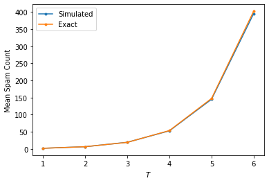
Finally, we plot the data from the table above to show the good agreement between the simulated and exact results.
fig, ax = plt.subplots()
df_rslts.plot(ax = ax, x='T', y = 'simulated_mean_spam_cnt', marker='.', label='Simulated')
df_rslts.plot(ax = ax, x='T', y = 'exact_mean_spam_cnt', marker='.', label='Exact')
ax.legend()
ax.set_xlabel('$T$')
ax.set_ylabel('Mean Spam Count')
plt.show()