Bayesian Linear Regression

In this post, I will reproduce the figures from Section 3.3.1 of Bishop’s Pattern Recognition and Machine Learning. A notebook to reproduce the contents of this post can be found here.

Description

We’ll investigate a Bayesian approach to regression and replicate some figures from a popular textbook.

We will collect noisy data of the form \((x_i,y_i)\) where the \(y_i\) are noisy measurements generated from a linear model with the following form:

\[y(x,w) = w_0 + w_1 \cdot x\]

The noise model is i.i.d. Gaussian with the form \(\mathcal{N}(0,\beta^2)\).

Our goal will be to estimate the true weight \(w\), and we will due this using a Bayesian approach. To do this, we suppose initially that the true weight came from a zero mean isotropic Gaussian distribution with known precision \(\alpha\). As we observe data, we will use Bayes theorem to update the posterior distribution (the formulas for the priors are given below). As we observe more and more data, the posterior will become increasingly concentrated on the true weight. We’ll demonstrate this by showing both the posterior distribution and sampling lines from the posterior distribution.

Note: As a short hand, I’ll refer to the parameter \(w\) as a linear weight. Also, I ignore Bishop’s convention for the target values, and use \(y\) in place of \(t\).

import matplotlib.pyplot as plt
import numpy as np
from scipy.stats import multivariate_normal 
from mpl_toolkits.mplot3d import Axes3D
from matplotlib import cm

%matplotlib inline

def y_w(x, w):
    return w[0] + w[1] * x

def noisy_data(x, a, beta):
    y = y_w(x, a)

    try:
        return y + np.random.normal(0, 1.0/np.sqrt(beta), len(x))
    except:
        return y + np.random.normal(0, 1.0/np.sqrt(beta))        

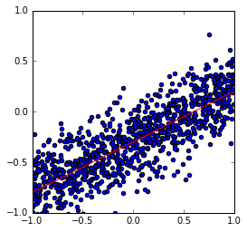
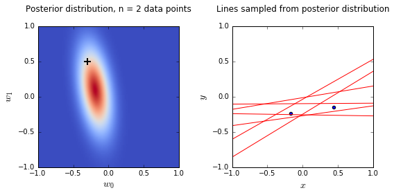
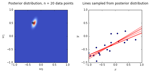
The true model has the linear weight \(w = (-0.3,0.5)\), i.e. an intercept of \(-0.3\) and slope of \(0.5\). We assume that the noise precision parameter is \(\beta = 25\).

# true linear weight:
w_true = np.array([-0.3,0.5])

# set seed for reproducibility:
np.random.seed(1)

# generate random (x,y(x,a)):
xs = np.random.uniform(-1.0, 1.0, 1000)
beta = 25.0
ys = noisy_data(xs, w_true, beta)

A plot of the true model (in red) along with the data samples.

# true line:
x_plot = np.linspace(-1.0, 1.0, 10)
y_plot = w_true[0] + w_true[1] * x_plot

# plot the true line and the data:
plt.scatter(xs, ys)
plt.plot(x_plot, y_plot, c='r')
plt.axis([-1, 1, -1, 1])
plt.axes().set_aspect('equal')

Prior Model

As I mentioned above, our prior on the linear weights \(w\) is a zero mean isotropic Gaussian distribution.

Specifically, our prior on the linear weights has the form:

\[p(w | \alpha) = \mathcal{N}(0, \alpha^{-1} I),\]

where the parameter \(\alpha > 0\). In Chapter 3 of Bishop’s book, he doesn’t explain how you would go about choosing \(\alpha\), so we will just suppose (as he does) that \(\alpha=2\).

alpha = 2.0

Posterior Distribution

Under the noise model and prior described above, it can be shown that when \(N\) data points have been observed the posterior distribution is Gaussian and given by:

\[p(w|y) = \mathcal{N}(w | m_N, S_N),\]

where

\[m_N = \beta S_N \Phi^T I,\]

and

\[S_N^{-1} = \alpha I + \beta \Phi^T \Phi.\]

Let’s create a random variable to simulate sampling from the posterior distribution:

# RV of posterior distribution on weights:
def ws_posterior_rv(N, xs = xs, ys = ys, alpha=alpha, beta=beta):
    # feature transformation:
    Phi = np.array([[1, x] for x in xs[:N]])
    
    # inverse covariance of posterior distribution:
    SNinv = alpha * np.eye(2) + beta * np.dot(Phi.T, Phi)
    SN = np.linalg.inv(SNinv)
    
    # mean of posterior distribution:
    if N > 0:
        mN = beta * np.dot(SN, np.dot(Phi.T, ys[:N]))
    else:
        mN = np.array([0,0])
        
    return multivariate_normal(mN,SN)

Plotting Function for the Examples Below

Now we write a convenience function to plot the posterior distribution for a data set of size \(N\). We’ll plot (and interpret) the dependence of the posterior distribution on the amount of used data below.

def plot_posteriors(N, xs = xs, ys = ys, N_ws = 6):
    w_posterior = ws_posterior_rv(N, xs, ys)
    ws = w_posterior.rvs(N_ws)
    
    nx = 100
    ny = 100 
    xg = np.linspace(-1,1,nx)
    yg = np.linspace(-1,1,ny)
    ps = np.array([[x,y] for x in xg for y in yg])
    
    xg = ps[:,0].reshape((nx,ny))
    yg = ps[:,1].reshape((nx,ny))
    zg = w_posterior.pdf(ps).reshape((nx,ny))
    
    fig, (ax0,ax1) = plt.subplots(1, 2)
    fig.set_size_inches(8,4)
    ax0.imshow(zg.T, interpolation='bilinear', origin='lower', 
               cmap=cm.coolwarm, extent=(-1, 1, -1, 1))
    ax0.scatter(w_true[0], w_true[1], c='black', marker='+', 
                s=100, linewidths=2.0)
    ax0.axis([-1,1,-1,1])
    ax0.set_xlabel(r'$$w_0$$', fontsize=14)
    ax0.set_ylabel(r'$$w_1$$', fontsize=14)        
    ax0.set_aspect('equal')
    ax0.set_title('Posterior distribution, n = {0} data points'.format(N), y = 1.08)
    
    ax1.scatter(xs[:N],ys[:N])
    for i in range(N_ws):
        y_plot = y_w(x_plot, ws[i,:])
        ax1.plot(x_plot, y_plot, c='r')
    ax1.axis([-1,1,-1,1])
    ax1.set_xlabel(r'$$x$$', fontsize=14)
    ax1.set_ylabel(r'$$y$$', fontsize=14)
    ax1.set_title('Lines sampled from posterior distribution'.format(N), y =1.08)    
    ax1.set_aspect('equal')
        
    #fig.subplots_adjust(hspace=-1)
    plt.tight_layout()
    return fig

Plots

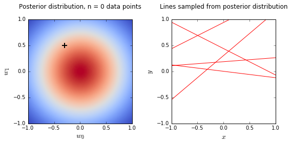
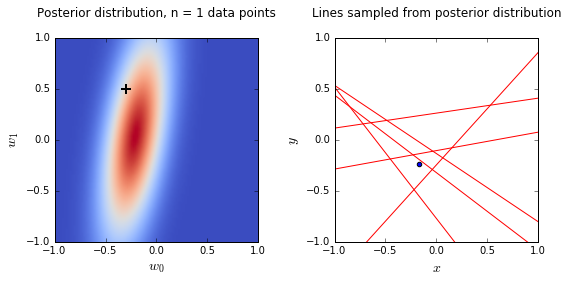
• On the left is a plot of the posterior distribution when we have observed \(N = 0,1,2,20\) data points. The \(N = 0\) case corresponds to the prior.
• We plot the true weight as a black cross on top of the posterior distribution.
• On the right is a plot of \(6\) lines generated from sampling linear weights from the posterior distribution.
• In addition to the lines sampled from the posterior distribution, we plot the \(N\) observed data points which were used to update the posterior distribution.

# set seed for reproducibility:
np.random.seed(10)

# generate analogous plots to Bishop Chapter 3:
for i in [0,1,2,20]:
    plot_posteriors(i)

What’s going on here?:

• we see that as the number of observations grows, the posterior distribution gets more confident about the solution and tends towards a delta centered approximately on the correct linear weight
• as a result, the lines sampled from the posterior distribution are converging toward a single line (with the approximately correct weight) as the number of observations gets large.

Let’s note that this wouldn’t be the case if we used a wildly bad choice for (\alpha). In fact, (\alpha) works as a regularizing parameter, and choosing too large a value for (\alpha) will bias the solution. (Essentially, Bishop gave us a decent (\alpha)).

A gif Demonstrating the Process

Since we have both a dynamic medium and more space than Bishop did, let’s generate a gif image to demonstrate the process. We’ll generate png images for (N = 0,1,\ldots,99) and I will use these to string together a gif image later.

%%capture
import os
try:
    os.mkdir('./imgs')
except:
    pass

# set seed for reproducibility:
np.random.seed(33)

# plot the images:
for i in range(0,100):
    fig = plot_posteriors(i, xs, ys)
    fig.savefig('./imgs/test_{0:03}.png'.format(i))
    fig.clf()

Here’s the gif that I made “later.”