In this post, we consider a sports league transitioning from their old draft pick strategy, where teams picked in reverse order to their win rank in the last season, to a new draft pick strategy based on rolling a \(T\) sided die to assign teams to \(T\) groups. These groups are ordered, with teams in the first group getting to pick before those in the second group and so on. Within each group, draft pick orders are assigned using the old strategy.

The motivation in this post is to solve the FiveThirtyEight “classic” riddler problem posted here. I’ll work out the solution to the problem and then simulate my results as a sanity check.

The code which generated this post can be found as a Jupyter notebook.

The prompt:

You are one of 30 team owners in a professional sports league. In the past, your league set the order for its annual draft using the teams’ records from the previous season — the team with the worst record got the first draft pick, the team with the second-worst record got the next pick, and so on. However, due to concerns about teams intentionally losing games to improve their picks, the league adopts a modified system. This year, each team tosses a coin. All the teams that call their coin toss correctly go into Group A, and the teams that lost the toss go into Group B. All the Group A teams pick before all the Group B teams; within each group, picks are ordered in the traditional way, from worst record to best. If your team would have picked 10th in the old system, what is your expected draft position under the new system?

Extra credit: Suppose each team is randomly assigned to one of T groups where all the teams in Group 1 pick, then all the teams in Group 2, and so on. (The coin-flipping scenario above is the case where \(T = 2\).) What is the expected draft position of the team with the Nth-best record?

Analytic Solution:

Some notation:

\(N\) to denote the order we would have been assigned in the old draft, this is 10 in the problem statement, but I’ll keep it general
\(D_N\) to represent the draft pick we get in the new system (when we would have been picked \(N^{th}\) in the old system).
\(M\) denotes the total number of teams
\(T\) denotes the total number of groups
\(A_i\) represents both the \(i^{th}\) group and the event that we are to the \(i^{th}\) group
\(N_{A_i}\) denotes the number of teams assigned to group \(A_i\)
\(n_{A_i}\) denotes the number of teams within group \(i\) that get to pick before us, (when we are assigned group \(i\))
\(P_i\) denotes the probability of getting assigned to group \(A_i\). Note: I keep the probabilities general here, allowing for a loaded \(T\) sided die, but will switch to the fair die below.

Following along with the prompt, we see that if we are assigned to group \(A_i\), then our order \(D_N\) can be found by adding up the number of teams in groups \(A_1,A_2,\ldots, A_{i-1}\) (since they all get to pick before group \(A_i\)) and then adding our order within group \(A_i\)

So we see:

\[\begin{array}{cl} E[D_N] &= \sum_{i=1}^{T} E[D_N|A_i] \cdot P_i\\ &= \sum_{i=1}^{T} (1 + E[n_{A_i}] + \sum_{j = 1}^{i-1} E[N_{A_j}|A_i]) \cdot P_i,\\ \end{array}\]

and all we have to do is compute these terms.

Computing \(E[n_{A_i}]\)

Let’s say that we’ve been assigned to group \(A_i\). If a team in group \(A_i\) gets to pick before us, this means that they must have had a better pick than us in the old style ordering. There are \(N-1\) teams that would have picked before us under the old system. Each team gets assigned to group \(A_i\) with probability \(P_i\), so the number of teams that get to pick before us within group \(A_i\) is a binomial random variable with parameters \(n = N - 1\) and \(p = P(A)\). That is,

\[n_{A_i} \sim \text{Binomial}(P_i, N - 1).\]

Since the mean of a binomial random variable is just \(p \cdot n\), we find:

\[E[n_{A_i}] = (N - 1) \cdot P_i.\]

Computing \(\sum_{j = 1}^{i-1} E[N_{A_j} | A_i]\).

Each team is assigned to group \(A_j\) with probability \(P_j\), so after we have been assigned to group \(A_i\) there are \(M - 1\) remaining teams to be distributed across the remaining groups, and the number of teams assigned to group \(A_j\) will follow a binomial distribution with \(p = P_j\) and \(n = M - 1\). So:

\[E[N_{A_j} | A_i] = (M - 1) \cdot P_j,\]

hence

\[\sum_{j=1}^{i-1} E[N_{A_j} | A_i] = \sum_{j=1}^{i-1} (M - 1) \cdot P_j.\]

Putting it together (solution for a possibly loaded die):

\[\begin{array}{cl} E[D_N] &= \sum_{i=1}^{T} E[D_N|A_i] \cdot P_i\\ &= \sum_{i=1}^{T} P_i (1 + (N - 1) P_i + \sum_{j=1}^{i-1} (M - 1) \cdot P_j)\\ &= 1 + (N - 1) \sum_{i=1}^T P_i^2 + (M - 1) \sum_{i=1}^{T} \sum_{j=1}^{i-1} P_i P_j\\ \end{array}\]

Extra credit Riddler solution (the case of a fair \(T\) sided die):

In this case, \(P_i = 1/T\) for all \(i\) so the expression above simplifies:

\[\begin{array}{cl} E[D_N] &= 1 + (N - 1) \sum_{i=1}^T (1/T)^2 + (M - 1) \sum_{i=1}^{T} \sum_{j=1}^{i-1} (1/T)^2\\ &= 1 + (N - 1) \cdot (1/T) + (M - 1)/T^2 \cdot \sum_{i=1}^{T} (i-1)\\ &= 1 + (N - 1) \cdot (1/T) + (M - 1)/T^2 \cdot (T \cdot (T-1))/2\\ \end{array}\]

That is, \(E[D_N] = 1 + \frac{N - 1}{T} + \frac{M - 1}{2} \left(1 - \frac{1}{T}\right)\)

Solution to the Riddler (no extra credit):

The riddler problem is just a special case where we use a fair \(T = 2\) sided die (also known as a fair coin), so we can just plug into the general expression above. Also, we should plug in our old style draft pick order, \(N = 10\), and the number of teams in the league, \(M = 30\).

Then, our new expected draft pick is:

\[E[D_N] = 1 + \frac{10 - 1}{2} + \frac{30 - 1}{2} \left(1 - \frac{1}{2}\right) = 12.75\]

So, we can expect to get a worse draft pick this season.

Simulation:

%matplotlib inline
import numpy as np
import matplotlib.pyplot as plt

Implement the analytical solution described above, just for the fair coin.

def analytical_solution(T, order=10, n_teams = 30):    
    # order is D_old
    # n_teams is N

    return 1 + ((order - 1.0)/T) + ((n_teams-1)/2.0) * (1- 1.0/T)

Let’s quickly check that I added correctly (for the \(T = 2\)) case.

analytical_solution(T = 2, order = 10, n_teams=30)

12.75

Now we’ll simulate the process as a sanity check for the solution given above.

def simulate(T, n_runs, n_teams=30, order=10):
    draft_position = np.zeros(n_runs)    
    
    # only call the random number generator once:
    rvs = np.random.random_integers(1, T, n_teams * n_runs)

    # reshape to get all n_runs:
    rvs = np.reshape(rvs, (n_runs,n_teams))

    for idx in range(n_runs):
        # what is our assignment?
        assignment = rvs[idx, order - 1]

        # how many teams below us were assigned to lower number groups?
        n_lower_assignments = len(np.where(rvs[idx,:] < assignment)[0])
        
        # how many teams with lower order than ours are in our group?
        n_lower_in_group = len(np.where(rvs[idx,0:order-1] == assignment)[0])
               
        draft_position[idx] = 1 + n_lower_assignments + n_lower_in_group
    return draft_position    

Wrap comparisions up into a nice tidy little function:

def print_comparision(T, n_runs = 10000, order = 10, n_teams=30):
    simulated_draft_position = np.mean(simulate(T, n_runs, n_teams=n_teams, order=order))
    analytical_draft_position = analytical_solution(T, order=order, n_teams=n_teams)

    print 'T = {0}'.format(T)
    print 'Expected draft position (simulated) : {0}'.format(simulated_draft_position)
    print 'Expected draft position (analytical): {0}'.format(analytical_draft_position)

Let’s check that our analytical results agree with our simulations.

for T in range(2,11):
    print_comparision(T, n_runs = 100000)

T = 2
Expected draft position (simulated) : 12.74021
Expected draft position (analytical): 12.75
T = 3
Expected draft position (simulated) : 13.62009
Expected draft position (analytical): 13.6666666667
T = 4
Expected draft position (simulated) : 14.13053
Expected draft position (analytical): 14.125
T = 5
Expected draft position (simulated) : 14.46331
Expected draft position (analytical): 14.4
T = 6
Expected draft position (simulated) : 14.56901
Expected draft position (analytical): 14.5833333333
T = 7
Expected draft position (simulated) : 14.72993
Expected draft position (analytical): 14.7142857143
T = 8
Expected draft position (simulated) : 14.83664
Expected draft position (analytical): 14.8125
T = 9
Expected draft position (simulated) : 14.8764
Expected draft position (analytical): 14.8888888889
T = 10
Expected draft position (simulated) : 14.94364
Expected draft position (analytical): 14.95

Good! Our computations seem to agree with our analytical results pretty well.

Examining the distribution of draft picks:

Let’s check out how the distribution of our draft pick \(D_N\) changes when we change the number of groups \(T\) while keeping our old style draft order at \(N = 10\) and the number of teams \(M = 30\) constant.

We’ll simulate a lot of draft picks for each \(T\) and plot the corresponding histograms.

def plot_distribution(T, n_runs=10000, n_teams = 30, order = 10):
    draft_position = simulate(T, n_runs, n_teams=n_teams, order=order)    
    plt.hist(draft_position, bins= n_teams, range=[1,n_teams], alpha = 0.5)
    plt.title('Histogram of Draft Pick Frequencies (T = {0})'.format(T));
    plt.xlabel('Draft Pick');
    plt.ylabel('Frequency (count)');    

plot_distribution(2, n_runs = 100000); plt.show();
plot_distribution(3, n_runs = 100000); plt.show();
plot_distribution(4, n_runs = 100000); plt.show();
plot_distribution(100, n_runs = 100000); plt.show()

png

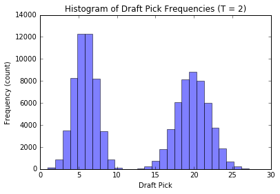
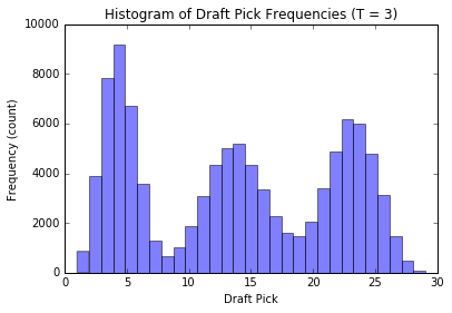
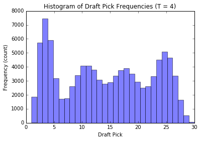
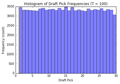
We see that when there are \(T\) groups, the histogram essentially follows a \(T\) modal distribution (see analytic discussion above, this is not unexpected, the reasoning is similar to our observations from before). Also, as \(T\) gets large, the distribution of our pick assignment tends toward a uniform distribution. Basically, the more groups to distribute the teams in, the less effect our old-style order has on the outcome, and our assignment becomes increasingly random.