Random Points on a Circle Riddler
Last week’s Riddler was about determining the probability that randomly distributed points on a circle all belong to a common same half-circle. It seemed like it should be pretty easy to solve by hand (edit: and it totally was), but for whatever reason I couldn’t piece out a solution. Instead, I settled for simulating the problem and making some pretty explanatory pictures.
Here’s the prompt copied verbatim from FiveThirtyEight for April 19:
If \(N\) points are generated at random places on the perimeter of a circle, what is the probability that you can pick a diameter such that all of those points are on only one side of the newly halved circle?
Determining When Points Belong to the Same Hemisphere
To simulate the solution, I used a simple geometric trick to detect when points lie in the same half-circle. Let \(C\) denote the unit circle in \(\mathbb{R}^2\). Then, \(p_1,\ldots, p_n \in C\) belong to the same hemisphere of \(C\) just in case there exists \(i \in \{1,\ldots,n\}\) for which either \(\min\left(\langle q_i, p_j \rangle\right) \geq 0\) or \(\max\left(\langle q_i, p_j \rangle\right) \leq 0\), where \(q_i\) is a non-zero perpendicular vector to \(p_i\).
To see that this works, note that the points \(p_k\) \(k=1,\ldots,n\) lie in the same half-circle iff we can split the circle \(C\) along a line \(l\) passing through the origin and one of the points \(p_i\), so that all points lie on the same side of \(l\). In turn, all points \(p_i\) lie on the same side of \(l\) iff they all share the same sign when projected onto a normal \(q_i\) to \(l\). Finally, note that \(q_i\) will be normal to \(l\) just in case \(q_i\) is perpendicular to \(p_i\) (since \(l\) passes through \(0\) and \(p_i\)). The following image shows how things work:

The function below uses this observation to determine whether angles \(\theta_i\), corresponding to points \(p_i\), lie in the same half-circle. It returns a tuple with a flag indicating whether a splitting line \(l\) exists (or not), and the index of the point \(p_i\) through which \(l\) passes. In the case that no split exists, it returns NaN in the second entry of the tuple.
import matplotlib.pyplot as plt
import numpy as np
%matplotlib inline
def thetas_on_same_half(thetas):
    thetas = thetas.flatten()
    n_thetas = thetas.size
    ps = np.array([np.cos(thetas), np.sin(thetas)]).T

    for i in range(n_thetas):
        q = np.array([ps[i,1], -ps[i,0]]).reshape((2,1))

        # be careful with the dot product p_i * q_i
        # this will only be zero to machine precision,
        # so it may be slightly positive or negative
        # make it actually zero to avoid this
        same_side_as_q = np.dot(ps, q)
        same_side_as_q[i] = 0.0

        proj_min = np.min(same_side_as_q)
        proj_max = np.max(same_side_as_q)

        if proj_min >= 0 or proj_max <= 0:
            return True, i
    return False, np.nan
Splitting Visualizations
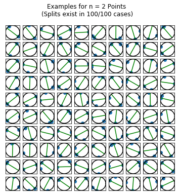
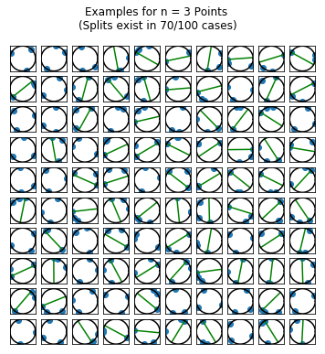
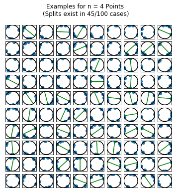
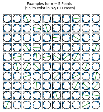
I wanted to get a sense (visually) of the frequency with which the points belong to the same hemisphere. So, I simulated 100 draws of \(n\) random points for \(n=2,\ldots,5\) points. For each draw, I plotted the points on a circle. If there was a line splitting the circle into a hemisphere containing all of the points and an empty hemisphere, then I drew the splitting line (in green) running through the point \(p_i\) described as above.
def plot_splits(n_points, n_row):
    n_runs = n_row*n_row
    thetas  = 2.0 * np.pi * np.random.rand(n_points, n_runs)
    results = np.zeros(n_runs, dtype='bool')
    idx = np.zeros(n_runs)
    ivals = []

    fig, axs = plt.subplots(n_row, n_row, figsize=(6,6))

    theta_circle = np.linspace(0, 2*np.pi, 1000)
    x_circle = np.cos(theta_circle)
    y_circle = np.sin(theta_circle)

    for i in range(n_runs):
        results[i], idx[i] = thetas_on_same_half(thetas[:, i])

    for i in range(n_runs):
        ax = axs[i % n_row, int(i / n_row)]
        if results[i]:
            idx_split = int(idx[i])
            theta_split = thetas[idx_split, i]
            x1, y1 = np.cos(theta_split), np.sin(theta_split)
            ax.plot([x1,-x1],[y1,-y1], c='g')

        ax.scatter(np.cos(thetas[:,i]), np.sin(thetas[:,i]), c='C0')
        ax.plot(x_circle, y_circle, c='k')
        ax.set_xlim(-1.01, 1.01)
        ax.set_ylim(-1.01, 1.01)
        ax.set_xticks([],[])
        ax.set_yticks([],[])
        fig.suptitle("Examples for n = {0} Points \n(Splits exist in {1}/{2} cases)".format(n_points,
                                                                             len(results[results == True]),
                                                                             n_runs))
    plt.show()
np.random.seed(797979)
for n_points in range(2, 5+1):
    plot_splits(n_points = n_points, n_row = 10)
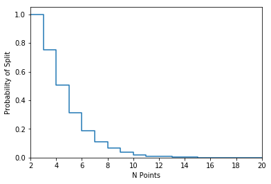
Simulating the Solution
Since I didn’t solve the problem analytically, the only thing I had left to do was to estimate the splitting probabilities for a range of different points. I estimated the probabilities for \(n = 2,\ldots,20\) points, using 25,000 draws of \(n\) random points for each \(n\).
def estimate_split_prob(n_points, n_runs):
    thetas  = 2.0 * np.pi * np.random.rand(n_points, n_runs)
    results = np.zeros(n_runs, dtype='bool')

    for i in range(n_runs):
        results[i], _ = thetas_on_same_half(thetas[:, i])
    p = len(results[results]) / n_runs
    return p
n_runs = 25000
n_points = np.arange(2, 20+1, dtype='int')
probs = np.zeros(n_points.size)

np.random.seed(797979)
for i, nps in enumerate(n_points):
    probs[i] = estimate_split_prob(nps, n_runs)
fig, ax = plt.subplots()
ax.plot(n_points, probs,drawstyle="steps-post")
ax.set_xlim(np.min(n_points), np.max(n_points))
ax.set_ylim(0, 1.05)
ax.set_xlabel("N Points")
ax.set_ylabel("Probability of Split")
plt.show()
print("N_pts\tProbability of Split")
print("-------------")
for i, nps in enumerate(n_points):
    print("{0}\t{1}".format(nps, probs[i]))
N_pts	Probability of Split
-------------
2	1.0
3	0.753
4	0.50792
5	0.31324
6	0.18852
7	0.11008
8	0.06452
9	0.037
10	0.01952
11	0.01088
12	0.00644
13	0.00312
14	0.00172
15	0.00076
16	0.0004
17	0.00028
18	8e-05
19	4e-05
20	0.0